Unit 23: Searching

Learning Objectives

After this unit students should be familiar with linear search and binary search algorithm, including understanding how the algorithms work, implementing the algorithms, arguing their correctness, and analyzing their running time.

Linear Search

Let's continue the discussion on efficiency on one of the fundamental problems in computing: how to look for something.

You have seen a similar problem in the problem Index in Exercise 3: Given a list of items \(L\) and query item \(q\), find if \(q\) is in \(L\).

Let's write a function to solve this. Our function returns -1 if \(q\) is not in the list. It returns the position of \(q\) in the list otherwise.

long search(long n, const long list[n], long q) {
  for (long i = 0; i < n; i += 1) {
    if (list[i] == q) {
      return i;
  }
  return -1;
}

What is the worst-case running time, expressed in Big-O notation, of the function above? Suppose the query \(q\) is not in the list, we will have to scan the whole list, once. The worst case running time is, therefore, \(O(n)\).

Can we do better? It turns out that this running time \(O(n)\) is also the best that we can do because we cannot be sure that \(q\) does not exist until we check every single element in the list. So there is no shortcut.

Binary Search

But, do we always have to check every element in the list? It turns out that, like many real-life situations, if the input list is sorted, we do not have to scan through every element. We can eliminate a huge chunk of the elements based on whether a chosen element is bigger or smaller than \(q\).

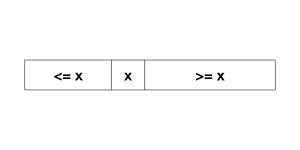
Suppose that the input list is sorted in increasing order. Pick a random element \(x\) from the list. Any element to the left of \(x\) must be less than or equal to \(x\), and any element to the right of \(x\) must be greater or equal to \(x\).

Suppose that \(q > x\), then we know that \(q\) must be to the right of \(x\), there is no need to search to the left of \(x\). Otherwise, \(q < x\), and \(q\) must be to the left of \(x\), and there is no need to search to the right of \(x\).

We can code this out using a recursive function below:

/**
 * Look for q in list[i]..list[j].
 *
 * @pre list is sorted
 * @return -1 if not found, the position of q in list otherwise.
 */
long search(const long list[], long i, long j, long q) {
  if (i > j) {
    return -1;
  }
  long mid = (i+j)/2;
  if (list[mid] == q) {
    return mid;
  } 
  if (list[mid] > q) {
    return search(list, i, mid-1, q);
  } 
  return search(list, mid+1, j, q);
}

We call this function with:

search(list, 0, n-1, q);

The search algorithm above is called binary search since it repeatedly cut the range of values to search by half.

Why is it correct?

It is not obvious at first glance that the code above correctly searches for \(q\) in \(L\).

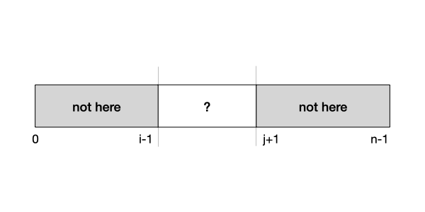
Let's analyze this function more systematically by writing an assertion for this function. What we want to do here is to eliminate elements in the array that cannot possibly contain \(q\) -- these are elements outside of the list[i] .. list[j] range. In other words, we want to assert that

// { q is not in list[0]..list[i-1] and list[j+1]..list[n-1] }

at the beginning of the function. In other words, this is a precondition for the function.

Let's see if this precondition is true at the beginning. Since \(i\) is \(0\) and \(j\) is \(n-1\), the ranges list[0]..list[i-1] and list[j+1]..list[n-1] are empty, so the assertion is true.

What happen if \(i > j\)? This implies that \(i - 1 > j - 1\), so the range list[0]..list[i-1] and the range list[j+1]..list[n-1] overlap. We can be sure that \(q\) is not anywhere in list.

Let's see how we ensure this assertion is true in the recursive call.

       :
  if (list[mid] > q) {
    return search(list, i, mid-1, q);
  } 
       :

Line 3 of the snippet above is invoked only if list[mid] > q. Since the array list is sorted, we know for sure that any element in list[mid+1]..list[j] is larger than \(q\). So, \(q\) cannot be anywhere in that range. We can assert, between Lines 2 and 3 above:

// { q is not in list[0]..list[i-1] and list[mid]..list[n-1] }

Thus, when Line 3 is invoked, the same assertion holds true. You can apply the same argument to the call:

  return search(list, mid+1, j, q);

To summarize, we annotate the code above with the assertions:

/**
 * Look for q in list[i]..list[j].
 *
 * @pre list is sorted
 * @pre q is not in list[0]..list[i-1] and list[j+1]..list[n-1]
 * @return -1 if not found, the position of q in list otherwise.
 */
long search(const long list[], long i, long j, long q) {
  if (i > j) {
    // { q is not in list[0]..list[n-1] }
    return -1;
  }
  long mid = (i+j)/2;
  if (list[mid] == q) {
    return mid;
  } 
  if (list[mid] > q) {
    // { q is not in list[0]..list[i-1] and list[mid]..list[n-1] }
    return search(list, i, mid-1, q);
  } 
  // { q is not in list[0]..list[mid] and list[j]..list[n-1] }
  return search(list, mid+1, j, q);
}

How Efficient is Binary Search

We have seen that if the input list is not sorted, then we minimally have to check every element in the list, leading to an \(O(n)\) algorithm.

With a sorted input and using binary search, however, we can do a better. Let's consider the worst case, where \(q\) is not in the list. Note that every comparison we make, we reduce the range of elements to search by half, until we reach one element. We start with \(n\) elements that could possibly contain \(q\). After one comparison, we are left with \(n/2\). After another comparison, we are left with \(n/4\), etc. It takes only \(O(\log_2 n)\) steps until we reach one element in the list. This is a big improvement over \(O(n)\) time: Suppose n is 1,000,000,000,000,000. Instead of scanning through and comparing one quadrillion elements, we only need to compare 50 of them!

Problem Set 23

Problem 23.1

(a) Write the code for performing binary search using loops. Identify the loop invariant and explain why the code works.

(b) Instead of returning the position of the query q, modify binary search such that it returns the insert position of q as described below:

• a position k, such that a[k] <= q <= a[k+1].
• -1 if q < a[0]
• n-1 if q > a[n-1]